2019. 12. 4. 14:53ㆍ학교공부/지능시스템
이번에는 categorial features에 대한 예측을 어떻게 수행할까에 대한 문제이다.
예제와 함께 살펴보자.

multivariable linear regression model의 기본 구조는 continuous descriptive features에서만 이용될 수 있다. 그래서 categorial descriptive features를 다루기 위해서 새로운 방법이 필요하다.
가장 널리 쓰이는 접근법은 single categorial descriptive feature를 a number of continuous descriptive feature values로 변환하는 방식이다.
예를 들어서, 위 예제의 Energe Rating은 세개의 continous descriptive features로 변형될 수 있다.

다시 예제로 돌아와서, 이 rental price에 대한 regression equation model은 다음과 같이 변했다.

하지만 이 접근법에는 문제가 있다.
1) 최적의 값을 찾기 위한 weights들이 새로 생겨버린다. 위 예제는 4 descriptive feature밖에 없는 매우 간단한 예제지만, 7개의 weights값이 필요하다.
2) training model을 search할 때 weight space의 크기를 증가시킨다.
3) 이러한 효과를 줄이기 위한 방법으로
- 각각의 categorial feature를 변환할 때, new features가 모두 0값을 가지면 original feature이 final level을 갖고 있다고 생각한다.
- 예를 들어 위의 ENERGY RATING feature에서, RAITING A,B,C를 다 넣는것 대신에 그냥 RATING A,B만 넣고, 둘다 0값을 가지면 ENERGY C를 implicitly set이라고 생각한다.
Handling Categorial Target Feature

여러개의 발전기에 대한 분석 결과 예제이다.
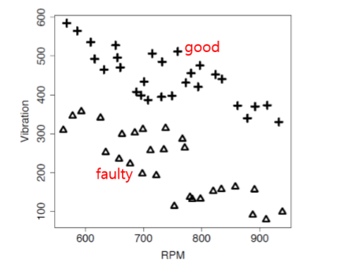
위 그림은 vibaration과 rpm에 대한 scatter plot이다. good generator은 +, faulty generator은 세모로 나타냈다.

경계가 비교적 뚜렷하고, decision boundary가 생성된다.
이 decision boundar는 linear seperator이고, 다음과 같은 수식으로 정의된다.

위 식을 이용해서 RPM=810, Vibration = 495인 generater를 예측하면,
계산결과는 830 - 0.667 * 810 - 495 = -205.27이며, decision boundary 위에 있다.
만약 RPM = 650m, Vibartion = 240이면, 값은 156.45로, boundary 밑에 있다.
* decision boundary 위에 나타나는 모든 data points들은 decision boudnary equation에 넣으면 모두 음수값이 되고, boundary 아래의 모든 datapoints들은 양수값을 가진다.
* 이 equation의 값들이 so well behaved이므로, 우리는 이를 categorial target feature을 예상하는데에 쓸 수 있다.
* 이전의 notation을 이용해서,

이 법칙을 이용해서 만들어진 surface를 decision surface라 한다.
그렇다면 어떻게 weights w값을 정할 수 있을까?
위 그림의 식에서 decision boundary는 불연속적이기때문에 미분불가능하다. 따라서 gradient로 error surface를 계산할 수 없다.
더욱이, 이 모델은 0 아니면 1이라는 매우 확실한 예측을 지닌다. a little more subtlety가 필요하다.
이러한 issue를 조금 정교한 threshold function을 만들어서 해결하고, 연속적이게 만들어 미분가능하고 subtlety desired로 만든다. 이는 logistic function이다.

이 logistic regression model을 생성하기 위해서는,

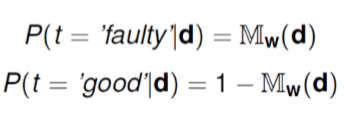
이 logistic regression model을 training하기 전에, 우리는 binary target level을 0 또는 1로 매핑한다.
그러면 각각의 인스턴스에 대한 이 모델의 error은 difference between target feature(0 or 1) and value of the prediction[0,1]이 된다.

이 Logistic Regression model 의 output은 target level이 나타날 확률로 평가될 수 있다.
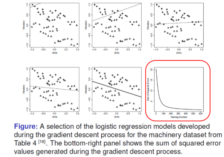
이 logistic regression problem에 대한 Optimal decision boundary를 찾기 위해서 gradient descent 알고리즘을 이용해서 SSE를 최소화 시킨다.
이 logistic regression model에서 gradient descent model을 새로 세운다.

증명과정은 복잡하므로 생략한다.
그럼 이제 다시 우리의 예제로 돌아오자. 다시 generator dataset이다.

다음과 같이 RPM과 vibaration간의 scatter plot이 나타나있다. good generator은 +, faulty generator은 삼각형 모양으로 나타나있다.
logistic regression model에서는 descriptive feature 값이 항상 normalized시킬것을 권장한다.
이 에제에서는, training을 시작하기 전 우선 두개의 descriptive feature에 대해 [-1,1]range로 normalize를 수행할것이다.
또한 learning rate alpha = 0.02로 세팅한다.

초기 가중치값은 다음과 같이 설정했다.

error delta function을 직접 계산해보자.