[지능시스템] 8장. Evaluation

 

Machine Leraning Model을 어떻게 평가할 수 있을까?

주의 할 점은 data used to evaluate the model은 data used to train the model과 같지 않아야 한다.

표준적인 Approach 방식은 hold-out test set이다.

hold-out test set은 랜덤으로 data의 일부를 sampling한 후 이 data는 training에 사용하지 않고, performace evaluation에 사용하는 방법이다.

예를 들어 보자.

Email classification with a binary cateogorial target feature(spam or ham)이 있다.

 

위 표에서 보듯이, 4가지의 가능한 Output이 있다. TP, TN, FP, FN이다.

1) TP(True Positive) : target set는 positive 값을 가지고, 예측 결과가 마찬가지로 positive임.

2) TN(True Negative) : target set는 negative값을 가지고, 예측 결과가 마찬가지로 negative임.

3) FP(False Positive): 인스턴스는 negative값을 가지나 예측결과는 positive로 잘못된 경우.

4) FN(False Negative): 인스턴스는 positive값을 가지나, 예측결과는 negative로 잘못된 경우.

위 이메일 예제에서는 다음과 같다.

가장 간단한 performace measure방식은 

classification accuracy는 반대로 0.75가 된다.

 

Model이 어떻게 performing되는지 완전히 이해하고 싶을 때, single performance beyond보다 더 많이 고려하는게 도움이 된다.

 

Designing Evaluation Experiments

: Hold-out sampling, k-Fold cross validation, Leave-one-out cross validation, bootstrapping, Out-of-time sampling

 

1) Hold-out Sampling

large datasets를 가질 때 적절한 방법이다.

그럼 위의 validation set은 어디다 써먹을까?

Validation set를 이용하는 이유는 overfitting을 방지하기 위함이다. ID3 알고리즘에서 decision tree를 만들거나 gradient descent algorithm에서 algorithm이 진행하면 진행할수록 모델이 오히려 overfitting되는 경우가 생긴다. 위 그림에서 보듯이 training iteration이 증가할수록 오히려 misclasification rate가 증가하는 것이다. 

따라서 우리는 validation test set를 통해 어느 지점에서 overfitting이 발생하는지 비교해볼 수 있다.

hold-out sampling에서는 두가지 이슈가 있다.

첫째로, hold-out sampling을 이용할 때는 enough data가 있어야 하고, 

둘째로, hold-out sampling으로 이용한 performance measurement는 우리가 lucky split을 만들경우 misleading할 수 있는 위험이 존재한다. 

 

2) K-Fold Cross Validation

이 방법에서는 available data가 k equal-sized folds로 분할되고, k seperate evaluation이 수행된다.

우리가 medical deicision making system을 만든다고 생각해보자,.

- 예측 system은 자동으로 orientation of chest x-rays를 결정한다(lateral or frontal).

- full dataset 500개를 기반으로, system 성능을 5-fold cross validation으로 예측할 것이다.

그러면 dataset은 다섯개 fold로 분할되고, 각각의 fold는 100개 instance를 가진다.

또한 5번의 evaluation experiments가 실행된다.

 

이제 aggregate confusion matrix를 만들 수 있다. 해당하는 cell의 모든 값들을 더해서 만들 수 있다.

 

3) Leave-one-out Cross Validation

: amount of data가 너무 작을 경우 useful한 방법이다. 이는 k-fold cross validation의 극단적인 버전이다.

여기서 k는 training instance의 수가 된다.

 

 

4) Bootstrapping

: 300인스턴스보다 적은 very small datasets에 적용된다. k-fold cross validation과 유사하다.

k개의 bootstrap sample이 생성된다. random sampling with replacement of n instances(n datasets)가 진행되고, 이를 k번 반복하는 식이다.

 

5) Out-of-time Sampling

: time dimension 차원을 이용한다.

data에서 one period를 training set를 생성하는데 이용하고, anothe rperiod에는 test set를 생성하는데 이용한다.

예를 들어서 customer churn scenario를 생성할 때, 이번년도의 customer behavior를 training set로 이용하고, 내년의 customer behavior을 test set로 이용하는 식이다. 이는 hold-out sampling의 형태로, out-of time sampling을 이용할 때에는 timing이 bias를 유도하지 않도록 해야한다.

 

2. Evaluation for Categorial Targets

이번에는 Cateogorial targets에 대한 evaluatiom을 알아보자.

1) Confusion Matrix-based Measures.

Confusion matrix는 위에서 살펴본 것과 같다.

여기서,

* TPR(true positive rate) : sensitivity라고도 불리며, TP / (TP + FN). 

* TNR(true negative rate): specificity라고도 불리며, TN / (TN + FP).

* FPR(false positive rate) : FP / (TN+FP)

* FNR(false negative rate) : FN / (TP+FN)

여기서 FNR = 1-TPR이고, FPR = 1-TNR이다.

위의 모든 measures들은 [0,1] 값이고, TPR과 TNR이 높으면 better performance를 의미,

FPR과 FNR이 낮으면 better peformance를 의미한다.

아까의 email classification 예제에서는,

 

2) Precision ,Recall, F1 Measure

* Recall은 true positive rate(TPR)과 같다.

: 이는 positive targe level을 가진 instance를 얼마나 잘 맞추는가를 의미한다.

recall = TP / (TP+FN)

더 높은 recall value는 better performance를 의미한다.

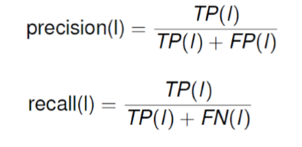
* Precision은 how often the positive prediction turns out to be correct([0,1])을 의미한다.

이는 positive target으로 예측된 값이 진짜 positive인가를 본다.

precision = TP / (TP+FP)

위의 email classificaition 예제에서는, recall = 0.667, precision = 0.75이다.

recall과 precision의 의미는,

- Precision : 1 - spam으로 표시된 email이 사실은 ham일 확률

- Recall : 1 - spam인 이메일이 시스템에서 걸러지지 못할 확률

 

위 precision과 recall을 한데 모아 평가할 수 있다. F1 measure

조화평균은 arithmetic mean에 비해서 large outliers에 대해서 덜 민감하다. (0,1]의 값을 가지며, higher values는 better performance를 의미한다.

위의 email classification 예제에서 recall = 0.667, precision = 0.75였으므로

F1-measure = 2 * (0.667 * 0.75) / (0.667+0.75) = 0.706

 

위의 precision, recall, F1-measure은 binary taregets에 대한 prediction problem에서 work best이다.

이 방법은 model의 성능을 positive target(or most important target)으로 평가하며, negative target에 대해서는 덜 강조한다. 이는 many applications에 유용한데, medical applications에서, patient가 질병이 있는지를 판단하는것이 질병이 없는지를 판단하는것보다 더 중요한게 그 예시이다.

하지만, 가끔 한 target level만이 중요하지 않을때가 있다.

위 예제에서는 test dataset이 imbalanced되었다.(90개가 non-churn이고 10개가 churn이다.)

이 문제를 해결하기 위해서 average class accuracy를 classcification accuracy 대신 쓴다.

그러면 위의 예제는 다음과 같이 변형된다.

위는 average class accuracies_AM for two models를 나타낸 것이다.

하지만 average class accuracy를 측정할 때 자주 arithmetic mean보다 harmonic mean을 이용하는것이 더 우선된다.

harmoic mean은  arithmetic mean보다 더 낙관적인 관점에서의 결과를 낸다.

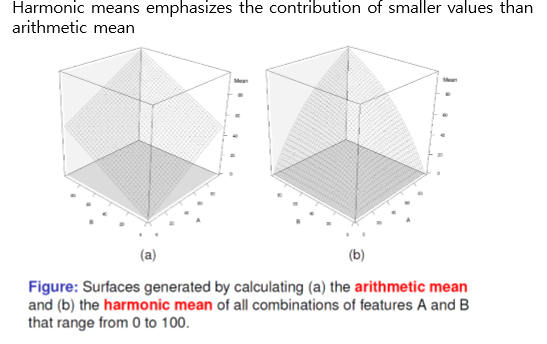
조화평균은 smaller values들의 기여를 arithmetic mean보다 더 강조한다.

위 예제의 조화평균 계산 결과는 다음과 같다.

 

지금까지의 performance measure방법은 data cell 안에 같은 가중치를 두고 평가했다. 하지만 항상 모든 결과를 동일한 가중치로 평가하는게 옳지는 않다. 이러한 경우에, cost of the difference outcomes를 고려해서 evaluating models를 만든다.

그렇게 만들어진 profit matrix는 다음과 같다.

예제와 함께 보자.

위의 표는 profit matrix이고, 아래는 각각 KNN model과 decision tree 모델에 대한 분석 결과를 나타냈다. 이를 profit matrix를 이용해 평가할것이다.

KNN model에서 prediction이 good이었는데 target이 good인 경우는 57. 따라서 57*140 = 7980

FN = -140 * 3 = -420

FP = -700 * 10 = -7000

TN = 30 * 0 = 0 이다.

 = 

총 계산 결과는 다음과 같다. 

이번에는 Multinominal targets에 대해 평가방법을 알아보자.

confusion matrix는 위 그림과 같이 생성되게 된다.

밑에 precision과 옆의 recall은 binary problems에서의 해석방법과 같다.

여기서 l 은 target level l이다.

예제와 함께 살펴보자. 박테리아 종을 분류하는 문제이다.

위 Table에 대한 confusin matrix를 만들면 다음과 같다.

recall(l) = TP(l) / (TP(l)+FP(l)) 이었으므로, 

recall(durionis) = 5 / 5+2 = 0.714

recall(ficulneus) = 6 / 6+1 = 0.857

recall(fructosus) = 10 / 11 = 0.909

recall(pseudo) = 3 / 5 = 0.6이다.

또한 Precision(l) = TP(l) / (TP(l)+FN(l)) 이므로,

Precision(durionis) = 5 / 5 = 1

Precision(ficulneus) = 6 / 7 = 0.857 ..등등이다.

Overall Classification Accuracy = 5+6+10+3 / 7+7+11+5 = 0.8이고,

Average class accuracy는 위 그림과 같이 계산할 경우 75%이다.

 

이번에는 Continuous target에 대한 evaluation 방법이다.

만약 prediction model이 continuous targets에 대해 예측해야 한다면, 몇 옵션들을 선택할 수 있다. 우리는 how accurately the predicted values match the correct targe values를 재는게 목표다.

 

1) Sum of Spread Error(SSE)

이 방법은 expected target values와 predicted values들의 차이를 모두 더한 값을 이용한다.

하지만 SSE는 test instance의 수가 증가할수록 SSE가 증가하는 경향을 띤다.

 

2) Mean Squared Error(MSE)

MSE방식은 average difference를 측정한다. MSE는 [0,infinite]까지의 value를 가질 수 있고, 더 작을수록 더 better model으로 평가된다.

예제와 함께 살펴보자.

위 예제는 drug dosage prediction을 측정하는 예제이다.

오른쪽의 평가 결과를 보면 Model 1의 MSE값이 더 낮으므로, Model 1이 Model2보다 더 예측 모델이 좋다고 평가된다.

MSE의 문제는 MSE 값들은 크게 의미있는 값이 될 수 없다는 것이다.

 

3) Root Mean Squared Error(RMSE)

RMSE는 error of prediction에 대해서 더 의미있는 정보를 제공한다.

 

4) Mean Absolute Error(MAE)

:

MAE에는 제곱 term이 없고 대신 abs를 쓴다(절댓값).

MAE는 [0,infinite]까지의 값을 가질 수 있고, 값이 작을수록 better model performance를 의미한다.

 

책에서는 RMSE를 더 많이 쓸 것을 제시하는데, 왜냐하면 performance of the models를 평가할 때 better to be pessimistic하기 때문이다. 

 

** Domain independent Err Measures

: RMSE와 MAE는 model성능에 대한 매우 직관적인 measure를 제시하지만, 몇 단점이 존재한다.

- domain에 대한 deep knowledge가 없을 경우, model이 정확한 판단을 내리는지에 대해 판단을 할 수 없음.

- 예를 들어서ㅡ RMSE가 1.38mg 값일 때 accurate prediction을 낸건지 아닌지 알 수 없다.

- 이러한 판단을 내리기 위해서, normalized, domain independent 평가 방법이 필요하다.

 

1) R^2 coefficient : domain independent measure

 

continuous target에 대한 평가방법으로 자주 이용된다. 위에서

total sum of square는

다음과 같다.

R2 coefficient는 [0,1)의 값을 가지고, 클 수록 좋다.