2019. 12. 3. 14:11ㆍ학교공부/지능시스템
Error-Based Learning에서는.
- parameterized된 model에 대해서 set of parameter의 대한 검색을 실시한다. 이 때, total error across the predictions made by the model with respect to a set of training intances가 최소화되는 set of parametrs를 찾는다.
- A paremetrized prediction model은 a set of random paremeters에 의해 intialized되고, error function은 이 초기 모델이 얼마 잘 수행되는지를 판단한다.
예제와 함께 살펴보자.

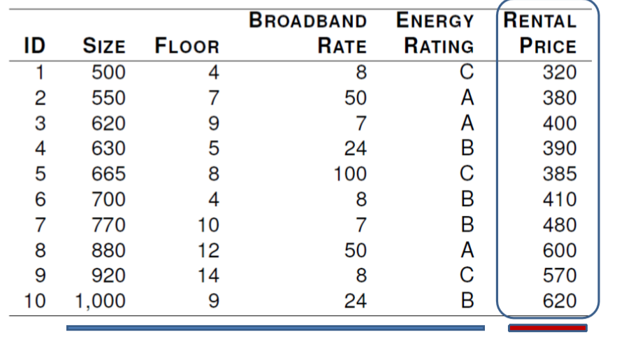
office rental price와 4가지의 descriptive features에 대해서 예측을 수행할 것이다.
처음으로는 ,SIZE를 이용해 Rental Price를 예측하고자하는 모델을 세운다.

이 dataset를 visualize하면,

두 feature사이의 상관관계를 확인할 수 있다.
우리가 이런 모델의 선형적인 관계를 찾을 수 있다면,
- office size가 rental price에 어떤 영향을 주는지 이해 가능
- office size에 대한 rental price 예측 가능
- new rental properties에 대한 rental price decision 가능
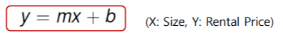
위 그림의 모델은 다음과 같이 표현된다.

즉 단순하게, Rental price는 6.47 더하기 0.62*SIZE가 된다.
이 모델을 이용해서, 730 square foot office에 대한 rental price를 예측하면,
Rental Price = 6.47 + 0.62*730 = 459.07이 된다.
이러한 종류의 모델을 Simple Linear Regression Model이라 한다.
우리는 이 Simple Regression Model을 다음과 같이 나타낼 수 있다.

여기서 중요한 key issue는, model의 weight w[0]과 w[1]을 어떻게 적절히 설정하느냐는 것이다.
-우리는 이를 error function을 정의함으로써 prediction output과 actual target values간의 error를 측정해서 결정한다.
즉, linear regression model을 a set of training model에 fit하기 위해서 error function(loss function이라고도 불림)이 필요하다.
가장 commonly used error function은 SSE function이다.

L2를 측정하기 위해서,
- Candidate model Mw를 이용해서 training set D의 각각의 member들에 대한 예측을 수행한다.
- 이러한 예측과 actual target values in the training set와의 error를 계산한다.
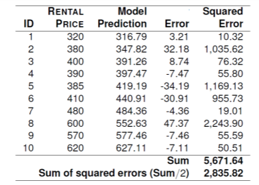
위 그림은 w[0]=6.47, w[1]=0.62로 설정한 후 예측한 결과이다.

왼쪽 그림은 3D surface plot을 나타낸 것이고, 오른쪽은 contour plot of the error surface를 나타낸 것이다. x축,y축은 각각 w[0],w[1]값이며, 모든 w[0],w[1]값의 조합에 대해서 sum of square error를 계산한 값을 나타낸 것이다.
그렇다면 어떻게 optimal weights를 찾을 수 있을까?
- 간단한 문제의 경우에는 단순히 brute-force search를 통해 찾을 수 있다. 하지만 실제 세상에서는 불가능하다. computationally expensive하기 때문.
- 그래서 combination of weights를 찾는 더 효율적인 방법이 필요하다.
- 예측 문제에 대해서, 위의 associated error surfaces는 두 가지 특성이 존재한다. error surfaces는 convex(마치 그릇 모양)이라는 것과, global minimum이 존재한다는 것이다.
error surface에서의 best point를 찾기 위해서, (global minmum), 우리는 이 point를 다음 식으로 정의한다.

이 point를 찾는데는 여러 방법이 있다. 우리는 guided search approach를 이용할 것이다.
*gradient descent algorithm*
error-based ML에서 가장 흔한 접근방법은 multivariable linear regression with gradient descent이다.
- 그렇다면 어떻게 gradient descent 방법이 linear regression에서의 optial weights를 찾을 수 있을까?
우리는 multivariable linear regression model을 다음과 같이 정의한다.

우리는 쓰레기 값(항상 1)을 지닌 descriptive feature d[0]을 위 식에 추가함으로써, 위 model을 간략화시킬 수 있다.

이제 위에서 언급했던 L2 function은 다음과 같이 단순화된다.

이제 예제와 함께 살펴보자.

위의 집값 예제를 다시 가져왔다.
이번에는 Size, floor, broadcast rate 세가지의 descritive feature에 대한 multivariable regression model을 생성할 것이다. 이 multivariate regression model의 식은 다음과 같다.

일단 나중에 best-fit set를 어떻게 만드는지 언급할 것이나. 일단 우리는 다음과 같이 weight를 설정할 것이다.

이 모델을 이용해서, Rental price를 위와 같이 나타냈다.
그래서 만약 690 square foot office와 11th floor, broadband rate of 50Mb per second인 지역에 대한 rental price 예측 결과는 다음과 같다.

1) Gradient Descent
Gradient Descent 방법은 아까 언급했듯이 다음 사실에 기반해 weights를 learning하는 접근법이다.
- error surfaces 는 convex shape이다.
- single global minimum이 존재한다.
우리는 guided search를 random starting position에서부터 시작할 것이다.

위 그림에서 하얗게 칠해진 점이 global minimum이다.
위의 office rental problem에서, SIZE와 RENTAL PRICE에 대한 관계는 다음과 같다.

multivariable linear regression models에 대한 Gradient descent algorithm은 다음과 같음.

D는 training instances의 수.
alpha는 learning rate. algorithm이 얼마나 빠르게 수렴하는지를 나타낸다.
errorDelta는 함수, weight w[j]를 어느 방향으로 조정할지 결정. error surface의 기울기를 dataset과 맞게 함.
alorithm을 끝내는 convergence 기준
위 알고리즘은 간단하게 말하면 w값이 convergence occurs를 할 때 까지 반복해서 w를 조정하는 알고리즘이다.

위 알고리즘에서 가장중요한 부분은 4번인데, weight가 update되는 부분이다.
각각의 weight값들은 독립적이며, weight에 작은 delta값을(errorDelta)더해주면서 조정한다.
이 조정은 change in the weight가 move downwards on the error surface임을 보장해야 함.

error delta는 어떻게 구하는 것일까?
만약 우리의 training set D가 just one training example(d,t)를 가진다고 생각해보자.
d는 descriptive feature이고 t는 target feature이다.
gradient of the error surface는 partial derivative of L2 with respect to each weight., w[j]가 된다.

위에서 3번째 식이 왜 4번째식이 되는지 살펴보자.
4가지 descriptive feature d[1],...,d[4]가 있다고 생각하자. d[0]는 dummy 값인 1이다.
dot product인 wd는 다음과 같게 된다.
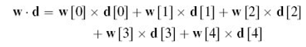
위 식에 대해서 w[0]에 대한 partial derivative를 수행하면 w[0] term을 제외하고는 다 0이 되므로,

w[4]까지 모두 동일한 방법으로 구한다.
t는 constant하므로 미분되면 0이 되므로 최종 값이 -d[j]가 되는 것이다.
그럼 이번에는 multiple training instance에 대해서 식을 세워보자.
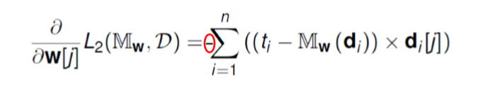
이 식을 error delta function으로 이용한다. 최종 gradient decsent algorithm은

w[j]는 any weight,
alpha는 constant learning rate,
ti는 expected target feature value for ith training instance,
Mw(d)는 weight vector w에 의해 정의된 예측 결과.,
d[j]는 jth descriptive feature of the ith training instance and corresponds with weight w[j]이다.
이를 직관적으로 이해해보자.
만약 error가 prediction outputs이 너무 크다고 판단하면
-> w[j]는 d[j]가 positive일 경우 감소하고,
-> w[j]는 d[j]가 negative일 경우 증가한다.
만약 error가 prediction outputs이 너무 작다고 판단하면
-> w[j]는 d[j]가 positive일 때 증가하고,
-> w[j]는 d[j]가 negative일 때 감소한다.
multivariable linear regression model에 대한 training 접근 방식은 batch gradient descent이다.
알고리즘의 iteration마다 각 weight에 one adjustment만 이루어진다.
* stochastic gradient descent
: 각각의 weight에 대한 조정이 each training instance individually하게 이루어짐.
어떻게 learning rate alpha를 고를 수 있을까?
learning rate alpha는 각각의 weight에 조정될 size of the adjustment를 결정한다.
하지만 learning rate를 고르는것은 well defined science가 아니다.
많은 예측은 경험법칙(trial and error)에 의해 이뤄짐.
A typical range for learning rates는 [0.00001, 10]임.

Learning rate가 너무 크면, global minimum을 찾지 못할 수도 있다.
1) (a)처럼 learning rate가 너무 작음
: 예측하는데 너무 오래 걸린다. 각각의 iteration마다 아주 작은 change가 이뤄지기 때문.
2) (c)처럼 너무 큰 learning rate
: global minimum을 놓칠 것이다. 알고리즘은 global minimum에서 jump back and forth를 반복할 것이다. 이는 SSE가 감소하기보다는 오히려 증가하게 만들고, process는 수렴하지 않을 것이다.
(3) (b)처럼 잘 정해진 learning rate
: 빨리 수렴하며, global minimum에도 도달한다.

예측할때는 주로 높은 값으로 먼저 예측해서 결과 그래프를 확인한다.
만약 결과 그래프가 (f)처럼 보이면 더 작은 value로 test시킨다.
이번에는 어떻게 initial weight를 정하는지 살펴보자.
Initial weight는 predefined range에서 랜덤적으로 고른다.
이 range를 선택하는것은 gradient descent algorithm이 얼마나 빠르게 수렴할지에 영향을 미친다.
initial weight를 고르는 것에 well-established, proven methods는 존재하지 않는다.
normalization을 통해서 initial weights를 좀더 쉽게 선택할 수 있는데, weight range가 normalized feature values에 대해서는 더 잘 정의되기 때문이다.
경험적인 법칙으로., [-0.2,0.2]사이의 initial weights를 고르는것이 잘 수행된다.
이제 예시와 함께 보자.
office rentals dataset를 continuous descriptive features로 예측할 것이다.

alpha와 weight에 대한 초기세팅을 수행했다.
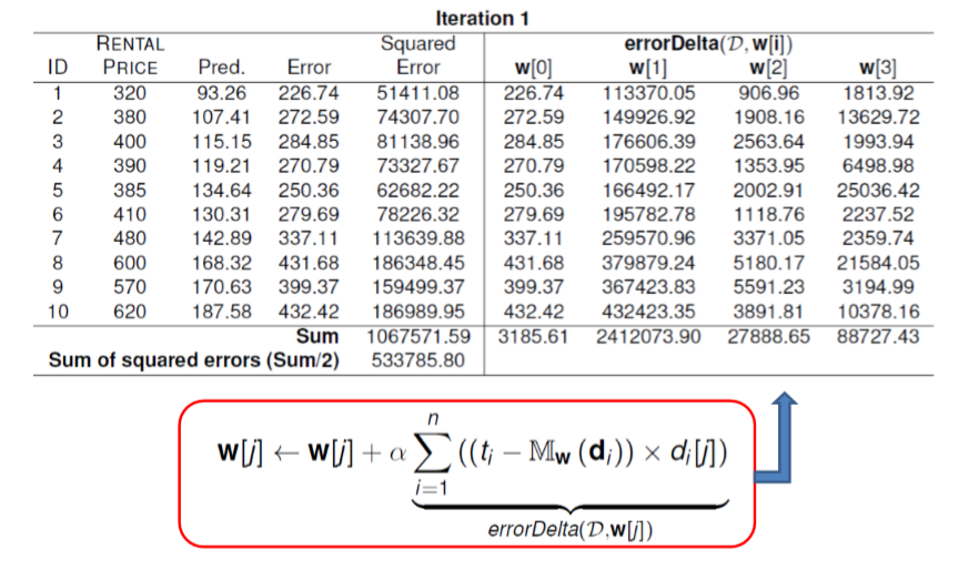
Squared Error = Error^2 = 266.74^2 = 51411.08
272.59^2 = 74305...로 계산된다.
error Delta(D,w[i])는
226.74 * 500 = 113370
272.59 * 550 = 149926 ..등등으로 계산된다.
첫번째 iteration에 대한 결과는 다음과 같다. 이제 weight를 error delta function을 이용해 조절한다.

w[2] <- -0.044 + 0.00000002 * 27888.65 = -0.043
w[3] <- 0.119 + 0.00000002 * 88727.43 = 0.121
으로 계산된다.
이제 새로운 weight에 대해 iteration2 를 수행한다.


알고리즘은 계속해서 weight update를 수행하고 이것이 수렴할 때 까지 수행한다. 100번의 수행 끝에 weight는,

다음과 같아진다. 이는 2913.5의 SSE값을 가진다.처음의 533만보다는 엄청나게 많이 개선됨,
그렇다면 이 예제에서의 alpha는(0.00000002) 왜 이렇게 낮은 값으로 설정했을까?
왜냐하면 RENTAL PRICE feature의 값이 [320,620]사이였기 때문에, 이는 error delta values를 너무 크게 만들었다.
따라서 normalization을 수행해서 이런 문제를 해결할 수 있다.
이를 파이썬코드로 구현하고 돌려봄.
|
1
2
3
4
5
6
7
8
9
10
11
12
13
14
15
16
17
18
19
20
21
22
23
24
25
26
27
28
29
30
31
32
33
34
35
36
37
38
39
40
41
42
43
44
45
46
47
48
49
50
51
52
53
54
55
56
|
f = open("gra.txt","r")
while(True):
line = f.readline()
if not line: break
x,y,z,t = map(int,(line.split()))
print(x,y,z,t)
count+=1
l1.append([x,y,z,t])
w_l = [-0.146,0.185,-0.044,0.119]
RP_l = []
diff_l = []
for k in range(2):
for i in range(count):
RP = w_l[0] + w_l[1]*l1[i][0] + w_l[2]*l1[i][1] + w_l[3]*l1[i][2]
RP_l.append(RP)
diff_l.append(abs(l1[i][3] - RP))
#print(RP_l)
#print(diff_l) # ti - Mw(di)
#sum of squared error
SSE_l = [x ** 2 for x in diff_l]
#print(SSE_l)
SSE = sum(SSE_l)/2
#print(SSE)
errorDelta_l = []
errorDelta_l.append([x for x in diff_l])
#print(errorDelta_l)
for i in range(3):
l3 = []
for j in range(10):
l3.append(diff_l[j]*l1[j][i])
errorDelta_l.append(l3)
#print(errorDelta_l)
w_sum = []
for i in range(len(w_l)):
w_sum.append(sum(errorDelta_l[i]))
#print(w_sum[i])
for i in range(len(w_l)):
w_l[i] = w_l[i] + alpha * w_sum[i]
#print(w_l[i])
RP_l = []
diff_l = []
for i in range(len(w_l)):
print(w_l[i])
|
cs |
gra.txt에 위 dataset가 들어간다. 2번 수행하면 위 책의 결과와 같게 나오나
100번 수행하면 overfitting된다. 책이 거짓말한건가? 아니면 내 코드가 잘못된것이다.

n번의 iteration에 대해서 SSE를 구해봤는데 n이 30~35일때 최저였다. 이후는 오히려 SSE가 증가했다.
n=33일 때,

weight는 이와 같다.
혹시 내가 잘못했을까 싶어 책의 weight를 초기값으로 놓고 SSE를 구해보았다.

위 책의 예제의 백번째 iteration에서도 SSE가 엄청 작다는걸 확인하였다.
따라서 weight값에 대해서 정답은 없다는걸 알게 되었다. 또한, 계산의 아주 사소한 차이가 weight를 많이 변화시키게 된다는 것도 알게 되었다.

60번 수행해서 최저값, convex 구해 봄.